This chapter is devoted to one of the most interesting applications of non-parametric statistical
diagnosis, namely, to the analysis of the human brain's electrical activity (the electroencephalogram, or
EEG). The meaning and the features of the EEG, as well as the problems arising from the high
non-stationarity of the EEG signal, are reviewed. We present experimental results demonstrating the
application of the statistical diagnosis methods described in this book to the EEG, and discuss the
prospects for further development of the change-point detection methodology with the emphasis on
the estimation of coupling between different signal channels.
View page by page
It was demonstrated by physiologists as early as at the end of XIXth century that if two electrodes are applied to the surface of a mammalian brain a sensitive instrument can show continuous fluctuations of the electric potential difference between the two electrodes. These potentials were later proved to be the product of the superposition of the electrical activity of tens or hundreds of thousands of neuron cells (neurons) lying in the surface areas of the brain, which is called the cortex. Each such cell is an elementary electric generator. In a rest state a neuron always has a potential difference of about 70 mV between its internal content bounded by a membrane and the surrounding media. In the active state of the neuron, when it receives the information or transmits it to another neurons, the polarisation of the membrane decreases; when the cell activity is inhibited the trans-membrane potential increases. When the potential difference falls below a certain threshold it induces a quickly propagating self-excitatory process, resulting in the activation of other neurons. This is the mechanism of signal transmission in neuronal networks.
The power of a single neuron is not high enough to produce potential changes which can be registered at the brain's surface or, especially, at the surface of the skin, because the surrounding tissues and liquids are good conductors and shunt the currents produced by the neuron. But if thousands of closely located cortical neurons work in synchrony, the summed oscillations of their trans-membrane potentials can be recorded from the scalp. Thus by registering the electrical potential at the surface of the scalp one can watch the activity of the important cortical areas of the brain. This method was called electroencephalography, and the electric signal recorded by this method was called an electroencephalogram; for both the method and the signal the same abbreviation (EEG) is used. The EEG signal is derived from a number of electrodes applied to the scalp's surface at approximately equal distances. The positions and the number of electrodes depends on the specific goal of a research. In modern practice about 20 electrodes are used most often, but the number varies over a wide range, from 1--2 to 128, and even 256. The signal recorded from each EEG electrode is obtained, amplified and, usually, processed in a separate "channel"; therefore, one may speak about the EEG signal at a given electrode as well as in a given "channel".
More recently a related, but much more expensive, method, magnetoencephalography (MEG), was developed for recording the summed magnetic field of the neurons; the signal registered by this latter method is very similar to the EEG signal.
In the 1920s a German psychiatrist Hans Berger demonstrated, in a series of dramatic studies, the sensitivity of the EEG to various changes of the human brain's functional state, and therefore the high diagnostic value of the EEG. In particular, he found that such a simple action as closing the eyes gives rise to regular oscillations in the EEG, with a period about 0.1 s and almost sinusoidal in shape. These oscillations, which he called the alpha rhythm (a term generally accepted since that time), were most prominent over the occipital regions of the brain. During mental activity, in contrast, the oscillations in the EEG were faster and less regular, and their amplitude markedly decreased. High voltage slow waves were characteristic for the EEG in deep sleep and during anaesthesia.
On the basis of his analysis of EEG phenomena, Berger suggested that they are a superposition of a number of quasi-periodic components, which manifest themselves in the EEG to various extents dependent on the brain's current activity. This "polyphonic" metaphor, regardless to the "true" nature of the brain's electrical oscillations, turned out to be useful for the quantitative analysis of the EEG. Their spectral analysis therefore became one of the main tools for the estimation of the brain's state, not only in basic research but in clinical practice as well. It is useful for diagnosing traumatic brain injuries, brain tumours, epilepsy, the group of the "degenerative" diseases of the brain such as Alzheimer's disease and Huntington's Chorea, and, in some cases, even psychiatric disorders (depression, schizophrenia). A specific research area, pharmaco-electroencephalography, was established in the field of human evaluations of psychoactive drugs (Dumermuth & Molinari 1987; Fink 1984). In this area it was shown that each of the main classes of psychoactive drugs, such as anxiolytics, neuroleptics or psychostimulants, induce a specific pattern or profile of changes in the EEG frequency spectrum. Moreover, the high sensitivity of the EEG to pharmacological effects made it possible to predict the therapeutic outcome by the EEG responses to a single dose of the drug (Coppola & Herrmann 1987; Herrmann 1982). The use of the EEG was also advantageous in development of new drugs (Itil & Itil 1986; Kaplan et al. 1997d; Versavel et al. 1995), because the class to which a new drug belongs can be estimated by the pattern of EEG spectral changes.
More recently developed techniques for non-invasive studies of the human brain, such as X-ray computational tomography, positron emission tomography, and magnetic resonance imaging, give good estimates of the localization of structural and metabolic changes in the brain's tissue. These new techniques, however, can provide a temporal resolution of only seconds or even tens of seconds, whilst the elementary processes of the information processing in the brain, such as detection, recognition, memorizing of external signals and even more complex cognitive operations, short "thoughts", are of the order of hundreds of milliseconds (Lehmann et al. 1995; Poppel 1994; Weiss 1992). Since the changes of neuronal cell membrane potentials, as discussed above, underlie signal exchange between the neurons, they are absolutely synchronous with the dynamics of the brain's information processing. The fluctuations of the total potential of neurons registered at the surface of the head, therefore, follow the activity of neuronal networks without time lags. This is why the EEG remains the most efficient method for studying the basic mechanisms of homeostasis and information processing in the human brain.
The high temporal resolution and the low cost of EEG technology, as well as the feasibility of combining it with advanced tomographic techniques, ensured this method one of the leading positions for a long time in the rapidly developing assortment of instruments for brain research.
The EEG signal, nevertheless, has an important inherent feature, its high non-stationarity, which leads to severe loss of the actual temporal resolution of the method. The main methodological advantage of the EEG therefore is not realized. However, the low temporal resolution of the spectral methods, which are most extensively employed in an EEG analysis, is the result of the low temporal resolution of the methods themselves. The spectral methods used for an EEG analysis are naturally associated with averaging; the lower the stability of the EEG signal, the longer the epoch required for obtaining statistically consistent estimates. It is the fight against the high non-stationarity of an EEG signal that leads to the loss of the main advantage of the electroencephalography.
Thus, the old method of EEG needs to be enhanced by new mathematical
approaches in order to provide comprehensive extraction of features from EEG recordings for the better
understanding of basic mechanisms of brain activities and for better diagnostics of brain diseases.
A vast variety of approaches to the extraction of quantitative features from an EEG signal was introduced during more than 70 years of electroencephalography. As for any signal, it seems promising to elaborate a mathematical model of the EEG signal. However, mathematical models (Nunez 1995; Freeman 1992) and physiological findings linking the EEG to electrical activities of single nerve cells (Eckhorn et al. 1988; Gray et al. 1989) remain problematic, and no single model of EEG dynamics has yet achieved the goal of integrating the wide variety of properties of an observed EEG and single-cell activities (Wright & Liley 1995). Successful attempts were limited to autoregressive modelling of short EEG segments (for a review see Kaipio & Karjalainen 1997). Further significant progress in this direction can hardly be expected, because the dynamics of EEG depends on brain activities related to a very complex dynamics of various types of information processing, which is related to repeatedly renewed internal and external information; thus stationary dynamic equations evidently cannot adequately describe an EEG signal.
The application of non-linear dynamics (or deterministic chaos) methods to the problem of the description of an EEG was relatively successful (Jansen 1991; Roeschke et al. 1997; Pritchard & Duke 1992). This theory operates with ensembles of trajectories of dynamical systems instead of a single trajectory and uses the probabilistic approach for description of observed systems. However, methods of non-linear dynamics are based upon the hypothesis that the brain's electrical activity can be described by stationary dynamic models. Such a hypothesis is unrealistic in many cases.
One way or another, all approaches to the description of an EEG use probabilistic concepts. Therefore, statistical approaches seem to be the most feasible and theoretically satisfactory methodology for the quantitative analysis of the EEG signal up to now.
Early in the history of electroencephalography, in view of the demands for quantitative
estimation of the EEG signal the reasonable question of its statistical nature was risen. Norbert Wiener
proposed considering the EEG as a stochastic signal by analogy with the output characteristics of any
complex system (Wiener 1961). It was thought at that stage of the exploration
of EEG that the main
laws of the dynamics of the total EEG signal could be studied on the basis of its probability--statistical
estimations irrespective of the real biophysical origin of cortical electrical processes (Lopes da Silva 1981).
As a result, a considerable body of work appeared concerning the stochastic properties of the
EEG signal. The main conclusion was that the EEG may actually be described by the basic stochastic
concepts (in other words, by probability distributions), but only at rather short realizations, usually
not longer than 10--20 s, because the EEG turned out to be an extremely non-stationary process. The
variability of power of the main spectral EEG components, e.g., for successive short term (5--10 s)
segments, ranged up to 50--100 % (Oken & Chiappa 1988). It became clear that the routine statistical
characteristics could be computed for the EEG only after its prior segmentation into relatively
stationary intervals. This, in turn, required the development of techniques for the detection of the
boundaries between the stationary segments in the EEG signal. The first positive findings in this line
have not only directed the way for more correct estimation of the EEG statistical properties but,
more importantly, provided the initial foundation for the principally novel understanding of the EEG
temporal structure as a piecewise stationary process (Bodenstein & Praetorius 1977).
Nonstationary phenomena are present in EEG usually in the form of transient events, such as sharp waves, spikes or spike-wave discharges which are characteristic for the epileptic EEG, or as alternation of relatively homogenous intervals (segments) with different statistical features (e.g., with different amplitude or variance) (Lopes da Silva 1978). The transient phenomena have specific pattern which makes it possible to identify them by visual inspection easily in most cases, whereas the identification of the homogenous segments of EEG requires a certain theoretical basis.
To perform the computerized analysis of an EEG record, it is converted into digital form. This means
that a quanted process is constructed from the signal which is continuous in its original form. The
sampling (digitizing) rate typically lies between 60 and 200 Hz, allowing spectral estimating in the
traditional range from 1 to 30 Hz, which includes most of the prominent components of the EEG.
Accordingly, if about 50--100 samples are necessary for a sound statistical estimation, there is no sense
to check the EEG intervals with less than 0.5--1 s duration for stationarity. If the EEG requires
further fragmentation to obtain stationary segments, consistent statistical estimates for so short
segments could not be obtained and the question of their stationarity would be senseless.
Assuming that the duration of a minimal stationary interval usually is no less than 2 s, as reported in (McEwen & Anderson 1975), the procedure of EEG segmentation into stationary fragments would consist of four stages. At the first stage, an EEG recording is divided preliminary into equal "elementary" segments of 2 s length. Then, each segment is characterized by a certain set of features, e.g., spectral estimations. At the third stage, using one of the multivariate statistical procedures, the elementary EEG segments are ascribed to one of a number of classes accordingly to their characteristics. Finally, the bounds between the segments belonging to a same class are erased. Thus, the EEG recording is transformed into a series of segments within which the EEG parameters remain relatively constant. Each of these stationary segments is characterized by its specific duration and typological features. If the number of segment types in the real EEG is not too high, the idea of piecewise stationary organization of the EEG will offer explicit advantages over the alternative primary concept of the EEG as a continuous stationary stochastic process.
This "fixed-interval" approach to the EEG segmentation was used in early works concerned with EEG segmentation (Giese et al. 1979; Jansen et al. 1979; Jansen et al. 1981; Barlow 1985). The number of typical EEG segments really turned out to be restricted, not more than 15--35 for different EEGs (Giese et al. 1979; Jansen et al. 1979; Jansen et al. 1981), and the duration of the majority of segments did not exceed 4 s, which provided evidence for the piecewise EEG organization.
However, this segmentation method had a serious disadvantage that some of the fixed intervals should necessary fall on boundaries between the real stationary EEG segments. This led to the appearance of a variety of EEG fragments which contained transition processes and, hence, were not strictly stationary. In addition, the boundaries between stationary segments were defined rather roughly, with the accuracy no better than the duration of the fixed interval.
To overcome these disadvantages, it was necessary to develop a segmentation procedure including adaptation of the segment boundaries to the real positions of the transitions between stationary intervals. This methodology, called adaptive segmentation, was applied, in one form or another, in the majority of methods of the automatic detection of stationary segments in the EEG (Barlow 1985).
Let us now consider the main approaches to the adaptive segmentation of
the EEG signal.
In general terms, the procedure of adaptive segmentation could be based on the estimation of the
extent of similarity of an initial fixed interval of EEG with an EEG interval of the same duration
viewed through the time window running along the EEG recording. The similarity index will drop
sharply when the window runs over a segment boundary, giving a formal indication of the transition
to the following segment. The autoregressive methods, which predict the EEG amplitude at a given
moment by analysing a series of amplitudes at prior moments, seems to be adequate for this task.
The discordance between predicted and real EEG amplitude could be a sufficient indication of a local
nonstationarity (Bodenstein & Praetorius 1977; Jansen 1991).
The methods of predicting time series are based on the assumption that their stochastic nature is substantially confined by certain dynamic rules. In this case, if mathematical models could be fitted to these regularities, the EEG amplitude will be predicted with a certain accuracy for a number of successive samples. Beyond the stationary segment to which the model parameters were fitted the prediction error will sharply increase, thus signalling the termination of the foregoing segment and the beginning of the next one. For the initial portion of this next segment, new model parameters can be computed, and then search for the next boundary can be continued. Thus, the parameters of the mathematical model of the EEG become the key element in search for segment-to-segment transitions, and a correct choice of the EEG model is very important.
In the framework of this idea, the coefficients of Kalman filter were first used for the model EEG description. A decision about the boundary were made if a sharp change in at least one of 10 filter coefficients was observed (Duquesnoy 1976, cit. by Barlow 1985). More recently, the most advanced technique for the EEG simulation, linear extrapolation, was applied for the EEG segmentation. This technique was developed by N. Wiener as early as 1942 as a supplement for autoregression analysis (cit. by Bodenstein & Praetorius 1977) and applied for the EEG analysis in the late 1960s (for a review see Kaipio & Karjalainen 1997). In the framework of the autoregression model, the EEG amplitude at a given moment can be predicted, with some error, as a sum of several previous amplitude values taken with certain coefficients. The principle procedures of the EEG adaptive segmentation based on the autoregressive models of a rather low order were first developed by Bodenstein and Praetorius (1977) and then in various modifications were successfully used by other authors (Bodunov 1985; Aufrichtig et al. 1991; Jansen 1991; Sanderson et al. 1980; Barlow & Creutzfeld 1981; Creutzfeldt et al. 1985; see also Barlow 1985 for a review of earlier works). According to different authors, the number of segment types lied in the range 6 to 50, and the duration of a stationary segment varied, in general, from 1--2 to 20 s (Bodunov 1985; Barlow & Creutzfeld 1981; Creutzfeldt et al. 1985). Use of the multiple regression analysis employing computation of the contribution of each of the several model parameters made the segmentation procedure more correct. With this technique, the authors managed to detect the EEG segments associated with some mental operations. They reported a similar duration range (2--10 s) for the majority of stationary EEG segments (Inouye et al. 1995).
Although the algorithms of many of the EEG segmentation methods based on the regression analysis
were thoroughly elaborated, almost all of them operate with the empirically chosen threshold criteria.
This makes it difficult to compare the results of segmentation not only from different subjects but
even from different EEG channels in the same subject. In addition to the inevitable empirical
predetermination, the threshold criterion for EEG segmentation in these techniques has a more
serious disadvantage, i.e., the tuning of the threshold cannot be refined in accord with the changing
parameters of the EEG process. The autoregressive model with the time-varying parameters tested in
speech recognition (Hall et al. 1983) seems to be an appropriate solution for this
problem. Some attempts have been made to apply this approach to the EEG (Amir & Gath 1989; Gath et al. 1992).
However, in the lack of a priori knowledge about the law of the
variations of model parameters it was necessary to construct an additional model, which should
result, in the general case, in accumulation of even greater error.
The methods of EEG adaptive segmentation based of autoregressive modelling used the same technique of running comparison of the EEG parameters in the referent and tested intervals, which made it possible to view the EEG structure only through a fixed time window. This approach determined a single time scale for EEG heterogeneities and, thus, prevented the insight into the total EEG structure, just like only neighbouring mountain peaks can be seen in the view-finder of a camera, while the mountain chain relief, as a whole, escapes from the visual field. It is quite possible, however, that the EEG contains larger transformations which are superimposed on the local segment structure and corresponds to a segment description of the EEG signal on a larger time scale.
Close to the solution of this problem was the study (Deistler et al. 1986), where a type of the regressive EEG modelling was also used, like in the works discussed above. The method described in this paper was quite sensitive to find the time moment of the beginning of action of neurotropic drugs. The authors analysed the EEG power in alpha band (8--12 Hz) on the assumption that its dynamics in a stationary interval can be approximated by a simple linear regression of y = at + b type, where y is the power in alpha band computed in a short time window with number t. In this case, the problem of finding a boundary between two quasi-stationary segments was reduced to a well-developed statistical procedure of comparison between coefficients a and b for two linear regressions at both sides of the presumed boundary. The point of the maximal statistically significant difference between two regressions indicated the joint point between the largest EEG segments. The authors emphasised the ability of their method to find only the most pronounced change if there is a number of change-points in the EEG recording, which was important for the specific application area of the method (Deistler et al. 1986). The structural analysis of the EEG in more general terms was not the objective of their study, and this was probably the reason why they did not pay attention to the potential of the method in this area.
From our point of view, the change-point obtained just as they
described could be placed at the macroscopic level of the EEG
structural description. If a similar procedure was performed further
for each of the two detected segments separately, the segments
corresponding to more detailed structure of the EEG could be obtained. By
repetitions of such a procedure a description of the microscopic level
of the EEG segment structure could be provided. Thus, there were
prospects for the description of the structural EEG organization as a
hierarchy of segmental descriptions on different time scales (Kaplan 1998).
In principle, the parametric methods of adaptive segmentation makes it possible to describe adequately the piecewise stationary structure of the EEG signal. However, all these methods designed for the analysis of nonstationary processes are based on a procedure which may be applied only to stationary processes, namely on fitting a mathematical model (usually the autoregressive one). It is evident that accurate fitting of a model can be achieved only on a stationary interval. The longer the interval, the finer characteristics of the process can be represented by the model. But the longer the analyzed interval of the real EEG, the more probable the incidence of heterogeneities within it (see, for example, McEwen & Anderson 1975). If the model is constructed on a very short interval, it will be very rough and the results of segmentation based on the parameters of this model cannot be expected to be of high quality (Brodsky et al. 1998; Brodsky et al. 1999).
Thus, the parametric methods of search for quasi-stationary EEG segments carry a rather strong
contradiction: segmentation into stationary fragments is impossible without construction of an
adequate mathematical model, but such a model cannot be constructed without previous
segmentation. Moreover, since the EEG is a highly composite and substantially nonlinear process
(Steriade et al. 1990; Nunez 1995), the development of a
rigorous linear mathematical model adequately representing the EEG intrinsic nature is hardly
possible (Kaipio & Karjalainen 1997). The parameters of even the well-fitted EEG models (e.g.,
Kaipio & Karjalainen 1997; Wright & Liley 1995) thus cannot follow the essence of the processes
underlying the EEG (Lopes da Silva 1981; Jansen 1991) and inevitably make the procedure of EEG
segmentation substantially rough. This is why the development of nonparametric EEG segmentation
methods is undoubtedly of interest. Application of such methods do not require previous testing for
stationarity, since they are not associated with fitting mathematical models to a process but rather are
based on the analysis of its individual statistical characteristics.
Study (Michael & Houchin 1979) is an example of one of the first nonparametric approaches to EEG segmentation. The authors also used the technique of running window, but compared the referent and tested EEG intervals not by the parameters of the autoregressive model but rather by the autocorrelation function. The integral index of the relative amplitude and shape discrepancy between the normalized autocorrelation functions of the referent and tested EEG intervals served as a nonparametric test of their difference (Michael & Houchin 1979). The later modification of this technique, which used the calculation of the normalized sum of the squares of differences of five autocorrelation coefficients as a measure of spectral dissimilarity between the referent and tested windows, performed satisfactory with clinical EEG recordings (Creutzfeldt et al. 1985).
Indices of spectral expansion also belong to the nonparametric estimations of time series. The Fast Fourier Transform (FFT) was one of the techniques employed for the fixed-interval EEG segmentation discussed above. As we noted, the main disadvantage of this approach to segmentation was the lack of adaptability of segment boundaries to the actual piecewise stationary structure. It seems natural to apply the FFT to a running time window and a referent window and then compare the obtained spectral estimations, in analogy with the adaptive segmentation procedure employing autoregressive modelling. A very high variance of the single spectral estimations (Jenkins & Watts 1972) is a serious obstacle on this way. Nevertheless, the only work applied this approach (Skrylev 1984) did demonstrate that it is quite efficient. In this study, the author used the maximal ratio between the narrow-band spectral power estimations as a measure of EEG spectral difference in two jointly running windows (Skrylev 1984), which made the method sufficiently sensitive to the EEG transition processes. However, the lack of the analytical justification of the threshold conditions, which is characteristic also for most of the adaptive segmentation techniques, still remained. In study (Omel'chenko et al. 1988) the use of an empirical statistical test for the assessment of inhomogeneity of spectral estimations of two EEG intervals made possible the justification of the choice of the threshold for detection of spectral differences. However, this work was not developed in the direction of EEG segmentation.
Though the first attempts to apply the nonparametric approach for EEG segmentation were rather
successful, its further development was restricted by the apparent condition that, in each specific
case, a statistical EEG characteristic most responsible for the EEG segmental structure (expected
value, variance, other statistical moments etc.) is unknown a priori. Moreover, the development of a
specific technique of quasi-stationary segmentation for each of these statistics is necessary; therefore,
the task of nonparametric EEG segmentation would consist in exhaustion of a rather large number of
possible solutions.
A new technology of the nonparametric EEG segmentation was developed on the basis of the theory of detecting the sharp changes or change-points in time series with a clear-cut piecewise stationary structure (Brodsky & Darkhovsky 1993). The change-points determined in such a way in a continuous EEG recording are the markers of the boundaries between stationary segments of the signal. The algorithm was based on the method of detection of multiple change-points in a stochastic process, which is described in Chapter 3 and, in more detail, in Appendix. Using this method in the EEG segmentation technique, after its "tuning" in a numerical experiment on the EEG-like simulated signals, made it possible not only reliably detect the intersegmental boundaries, but also to estimate, for the first time, the confidence intervals of their positions within the tested EEG record (Shishkin et al. 1997; Kaplan et al. 1997c; Brodsky et al. 1998).
A starting point for the development of this technology was provided by the piecewise-stationary metaphor of the EEG, i.e., the assumption that any EEG recording is "pasted" from relatively homogenous (in statistical sense) pieces (segments). The transition intervals between such pieces are supposed to be of minor length, and therefore can be roughly treated as a point (a change-point). Each homogenous segment of the signal is assumed to correspond to a period of stable activity of some brain system; thus the transitions from one segment to another show the time moments of the switching of the neuronal network activity (Kaplan et al. 1995; Brodsky et al. 1999). One may also expect that the change-points can reveal the consecutive operations of neuronal networks, with different time scales according to parameters of the algorithm of change-point detection (Kaplan et al. 1997b). The covert dynamics of the operational activity of brain systems, which cannot be disclosed by usual methods of EEG analysis, now can be studied.
The next aim of the EEG segmentation is estimation of the characteristic features of brain operational activity. The emphasis here should be made on the method capacity to work with various EEG types, which may differ substantially by their spectral components. If this task were solved, the EEGs recorded under different mental loading, during different functional states (e.g., during sleep or awake states), under different medication, etc., could be compared quantitatively by rate (frequency) of change-point occurence. Variations of the change-point rate across brain sites could also be of special interest, because they may help to compare the degree of the involvement of these sites in brain operations (Kaplan 1998; Kaplan 1999).
The high interconnectivity of different brain sites offers another field of the application of change-point detection with respect to spatial domain. It seems to be highly probable that the order of appearance of different segments in EEG channels deriving the electrical signal from spatially different regions of the brain cortex is co-ordinated across the channels in a degree dependent on the functional co-operation of these regions. It seems possible that investigation of the coincidence of change-points would enable, for the first time, the direct estimation of the coupling of inherent elementary operations going on in different brain areas, instead of routine phase-frequency synchrony in the terms of correlation and coherency (Kaplan et al. 1995; Kaplan 1998). A qualitative description (see below) of this type of synchrony, which we call the operational synchrony, provides the means for a radically new insight into the co-operation of brain structures.
It was shown during the adaptation of the change-point detection methods for EEG segmentation, that the following type of diagnostic sequence is appropriate for this purpose: yτ(t) = x(t)x(t+τ), where x(t) is the routine EEG, τ = 0,1,... is a fixed time lag (Brodsky et al. 1998). The main reason to choose this diagnostic sequence was that the nonstationarity of the EEG signal generally results from variations in its spectrum or, what is the same - in its correlation function. The EEG could therefore be viewed as "pasted" from a large number of random stationary (by the correlation function) processes. As it was described in Chapter 1 (Section 1.4), these diagnostic sequences should be used for the reduction of the problem of detecting changes in correlation function to the problem of detecting changes in expected value. All the experimental results described below were obtained with a particular variant of this diagnostic sequence (referred to as basic diagnostic sequence): y0(t)=x2(t).
While developing the algorithm of change-point detection in the EEG, we also intended to make possible to assess all the levels of the hierarchy of segmental description of the EEG, with different time scales (see above Subsection 7.3.2). The estimation of change-points were made by stages. The most "powerful" change-point was detected first, providing a boundary between two large segments of the recording; then the procedure was performed for these segments, which were more homogenous than the total recording, and the change-points of second level could be found if existed. The division into smaller segments was proceeded this way, until all the resulted segments were found to be homogenous (without change-points) or shorter than a certain threshold corresponding to the minimal length of sequence required for consistent statistical estimates. In more detail the algorithm is described in Chapters 3, in this Chapter in Subsection 7.4.1, and in Appendix (see also Brodsky et al. 1998; Shishkin et al. 1997; Kaplan et al. 1997c; Brodsky et al. 1999).
The threshold for change-point detection in our method is a function of "false alarm" probability (the probability to detect a change-point which in fact not exists). The latter parameter is set in an explicit form (Brodsky & Darkhovsky 1993; Brodsky et al. 1998; Shishkin et al. 1997), which is especially important because, irrespective of a specific technology of detection, the results of change-point detection could be obtained only as probabilistic estimates. The use of "false alarm" probability not only enables a wide range of the adaptation of detection procedure to specific research tasks, but also makes possible the work with different time scales. By increasing the "false alarm" level, for example, one may tune the procedure for most prominent intersegmentary transitions and work with the macroscopic segmentary structure of the EEG. The lower false alarm level results in revealing more detailed, microscopic segmentary structure. The repetitive processing of the same signal with different thresholds will yield the outlines of the hierarchy of EEG segmental description (see above subsection 7.3.2).
The application of the method in neurophysiological studies demonstrated
its sufficiently high sensitivity in estimation of the dynamics of
structural changes in EEG related to cognitive processing (Kaplan et al. 1997c; Kaplan et al. 1998).
This section presents the results of the application of the methodology described in the previous section to real EEG signal. The EEG was obtained from human subjects following standard procedures. The subjects were volunteers; all of them gave an informed consent concerning their participation in the experiments. The EEG signal in each EEG channel was registered as a difference of the potential at one of the electrodes applied to scalp and the potential at two electrically connected "reference" electrodes applied to both earlobes (at these sites potential variations are relatively low). Two montages, 8-channel and 16-channel, were used, both in accordance to the standard scheme "10-20". Electrode positions will be shown at the figures illustrating the text below.
To estimate the effects of various brain states, the EEG was recorded when subjects performed different mental tasks and in the rest state, with eyes open or closed. The difference between eyes open and closed states was of special interest, because it greatly modify the alpha band of EEG signal, which was the main subject of the analysis for its sensitivity to mental loading, relatively high power in awake state (in most normal humans) and well time-structured dynamics.
The analog signal was digitized, usually with A/D ratio of 128/s, and processed off-line. The recordings were visually inspected, and only those which contained no large artefacts were used for the analysis. Each EEG channel was processed separately except the final stages of the analysis of change-point coincidence. In most cases, the EEG was bandpass filtered, usually in the alpha band (8--12 or 7.5--12.5 Hz), prior to the change-point analysis.
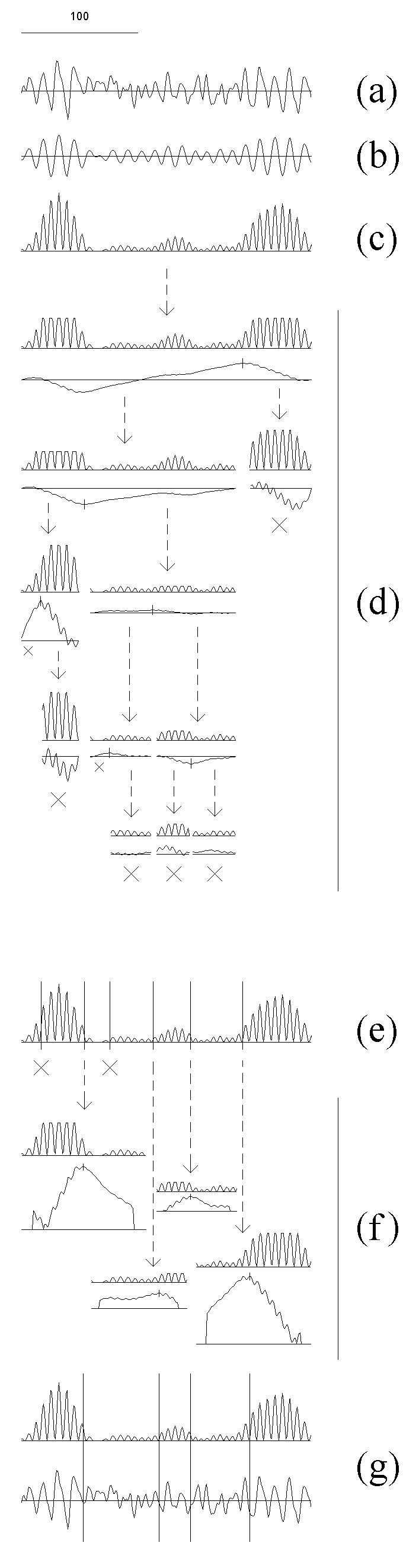
Fig. 7.1. Detection algorithm adapted for the EEG analysis
The EEG (a) was filtered in the alpha band (bandpass 7.5--12.5 Hz) (b) and then the
amplitude squared (c); the result is the sequence from which the subintervals
are cut out at further steps.
At the next stage (d) the initial interval is sequentially cut into subintervals
for which the homogeneity hypothesis is tested and the change-point instants
are preliminary estimated. In doing so, the outliers are rejected, and for
the resulting sequence (upper curve in each pair) the statistic YN(n,1)
(lower curve in each pair) and the threshold (not shown) are computed. The
threshold at this stage is computed with higher levels of the "false alarm"
probability: 0.4, 0.3 and 0.2 for subintervals with length
L, L ≥ 100, 50 ≤ L < 100 and 25 ≤ L < 50
samples, correspondingly. If the absolute maximum of the
statistic exceeded the threshold, its time instant becomes the preliminary
estimate of a change-point (vertical stroke on the curve), and the
subinterval is cut into two parts with an break off from it; otherwise the
subinterval is considered as stationary and is not analyzed further (large
crosses). Too short (less than 25 samples) subintervals also are not
analyzed (small crosses). The arrows show how the subintervals are cutting
out.
The obtained preliminary change-point estimates are re-examined (e) using
the statistic of the same type, but with lower "false alarm" probability,
0.2, 0.1 and 0.05 for subintervals
L ≥ 100, 50 ≤ L < 100 and 25 ≤ L < 50
samples, correspondingly. This results in rejecting of some change-points
(crosses).
At the final stage (f) the change-point instants are estimated precisely.
The subintervals for each of the survived change-points are defined with a
small break from the neighbouring change-points, and the outliers are
rejected in each subinterval separately (the upper curve in each pair). For
each subinterval, a statistic YN(n,0) (the lower curve in each pair)
is computed, and the time instant of its absolute maximum becomes the final
estimate of the change-point instant.
For illustrative purposes, the final change-points instants are shown against
the filtered and squared EEG, as well as the original EEG signal, by vertical
lines (g).
For more details of the algorithm see Chapters 3 and Appendix.
The sampling (digitizing) rate was 128/s (here and in the further figures, if
not specified). Horizontal scale: 100 samples. Vertical scales are in the
ratio of 1 (original and filtered EEG) : 250 (diagnostic sequences) : 25 (statistics).
Search for the change-point in power of one of the EEG spectral bands is illustrated in Fig. 7.1. An EEG recording (a) is digitally filtered (b) and transformed into the basic diagnostic sequence (c). The further stages are performed with subintervals of the basic sequence (for details see Chapters 3 and Appendix). In each subinterval the extreme values are "truncated", and then the statistic appropriate for the current stage is computed (Fig. 7.1, d and f). The recording is usually longer than shown at Fig. 7.1, and it can be divided previously into epochs (in our practice, from 200 to 2000 samples each) to be processed separately accordingly to the same schedule.
At the next preliminary stage (Fig. 7.1, d), the homogeneity hypothesis is checked, and preliminary change-point estimates are computed for the subintervals successively extracted from the basic diagnostic sequence. The following is done for each subinterval separately: the outliers are "truncated" on the basis of the distribution for the subinterval, then the statistic YN(n,1)and the threshold are computed (everywhere in this Chapter we use the statistics from the basic family (1.4.1)). For the calculation of the threshold at this stage, the "false alarm" probability is set at high level. If the maximum of absolute value of the statistic exceeds the threshold, its instant becomes a preliminary estimate of a change-point, and the subinterval is divided into two parts with receding from it; otherwise the subinterval is considered to be stationary and is not analysed further. Subintervals which are too short also are not analysed.
At the rejection stage (Fig. 7.1, e), for each preliminary change-point estimate a new subinterval is derived from the basic sequence receding from the change-point to each side by 0.9 distance to the neighbouring change-point. In this subinterval, the "truncation" is made, the statistic YN(n,1)is computed, and the change-point is checked using lower "false alarm" probability for the calculation of the threshold. Some of the change-points are rejected. At the final estimation stage (Fig. 7.1, f) the subintervals are formed in the same way (they may not differ from the subintervals formed at the previous stage at all, or some of them may become larger due to the rejection of some change-points). A different statistic, YN(n,0), is now calculated for each new subinterval, and the maximum of its absolute value becomes the final estimate of a change-point (see Fig. 7.1, f, g).
The EEG fragment shown in Fig. 7.1 exemplifies two features typical for the
EEG and its components: 1) the changes often are more or less gradual,
i.e., the EEG not completely corresponds to the piecewise stationarity model
and, thus, change-points indicated by a detection algorithm are not
always the estimates of actual change-points but also may mark non-instantaneous transition
processes; 2) even relatively short intervals may include more than one
change-points. Although the both features makes the problem of detection
more complicated, the procedure is able to divide the
EEG successfully into relatively homogenous segments, as is the case for
the fragment in Fig. 7.1.
We consider now change-points in different components of the frequency spectrum of typical EEG signal. An example given in Fig. 7.2 represents the following characteristic features of signal structure and results of change-point detection. Only few change-points in power are found in the initial EEG (unless a prominent alpha rhythm is present). Not many change-points are found after filtering in the bands of slow rhythm, called delta (b) and theta (c), which usually have no prominent time structure. The variations of the bandwidth usually not affect the number of detected change-points strongly. When slow rhythms make a considerable contribution to the total EEG power, its dynamics usually also has no clear time structure, and only few change-points could be found. After filtering in alpha (d) and beta (e) bands, on the contrary, a high number of change-points is found; the most clear modulations marked by change-points are in the alpha band. The relatively clear time structure of alpha activity is not a new fact, yet it is important to be mentioned because of high sensitivity of the alpha band to fine changes in brain state (Lehmann 1980). The change-points in this band therefore provide a useful tool for the brain state monitoring, and we concentrated on them most attention in our work.
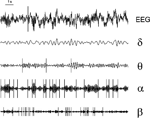
Fig. 7.2. Change-points in different frequency components of the EEG
EEG (subject tw12, eyes closed, no task) and the change-points
(vertical lines).
From the top down: the original signal; the signal
after digital filtering with bandpasses 3.5--7.5 Hz (theta), 8--12 Hz
(alpha) and 14--21 Hz (low beta). Change-point detection was made in
all these sequences (after squaring) with the same parameters. The
"false alarm" probability at the final stage of detection was 0.2
for intervals longer than 100 samples and 0.1 to 0.05 for shorter
intervals. The EEG was recorded from right occipital electrode (standard
position O2). Horizontal scale: 1 s.
The change-points in Fig. 7.2 follow the visually distinct modulations of the filtered signal, with no respect to a frequency band. Unfortunately, the "actual" position of a change-point in real EEG in most cases cannot be located. This is due to the lack of understanding of the EEG genesis; in particular, very little is known about the "events" in the brain tissues causing transformations of the dynamics of on-going EEG. Therefore verifying the detected change-points in the EEG is possible only on the basis of a standard method of change-point detection, which is currently unavailable. On the other hand, the experience of researchers and clinical electroencephalographists suggests that the visually distinct modulations of the EEG signal and its components are highly informative. This is why the visual control was found to be quite appropriate for the estimation of the quality of change-point detection.
Specifically, we inspected visually the EEG, both unprocessed and filtered, with the marks of the change-points detected in the alpha band power, which gives a sufficient impression of the correspondence of the detected change-points to the visible changes in the EEG alpha activity. This way we checked the validity of change-points found in 138 one-minute EEG recordings (7680 samples per recording), obtained from different subjects in various conditions. Although the automatic search for change-points was carried out in all the EEGs without any tuning of any parameters of the detection procedure, it was found that vast majority of detected change-points corresponded to real changes in alpha activity, and that most of visually distinct modulations of alpha activity were found by the program. Note that almost all the other known methods of EEG segmentation cannot work in such unsupervised regime and require the manual adjusting of the detection threshold for satisfactory detection of changes in EEG recordings with considerably different characteristics. In our program, the threshold was tuned completely automatically according to the "false alarm" probabilities defined for all the set of EEGs.
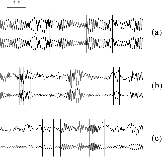
Fig. 7.3. Change-points in different types of the EEG alpha activity without substantial gradual changes
Change-points in different types of the EEG alpha activity without substantial gradual changes: (a) EEG with high amplitude, weakly modulated alpha rhythm (subject tw07); (b) EEG with well modulated alpha rhythm (tw09); (c) EEG with relatively low amplitude alpha rhythm (tw11). Upper and lower curves in each pair are original and filtered (7.5--12.5 Hz) EEG, correspondingly. EEG was recorded from right occipital electrode (O2) in eyes closed, rest condition. The vertical lines are the change-points detected in the basic diagnostic sequence. Horizontal scale: 1 s. (From Shishkin & Kaplan, in press).
Fig. 7.3 gives three examples of EEG representing various types of normal (physiological) alpha activity from our set of recordings. In the first example, the alpha rhythm makes main contribution to the total EEG; it has high power but is only slightly modulated. In the second example, the contribution of the alpha rhythm is also rather high, but it is strongly modulated and sometimes almost disappear. In the third example, the alpha band activity is at a low level most of time. As can be seen from Fig. 7.3, the program reliably detected the change-points despite of such variety of signal patterns.
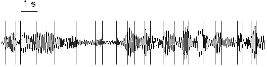
Fig. 7.4. Change-points in alpha activity (7.5--12.5 Hz) with gradual changes
Subject tw03, eyes closed, rest condition. Right occipital electrode (O2). The change-points (vertical lines) were detected in the basic diagnostic sequence. Horizontal scale: 1 s.
The changes of amplitude/power of the alpha rhythm in the EEG shown in
Fig. 7.3 were rather abrupt. Fig. 7.4 presents a more challenging type of
pattern, where abrupt changes in the alpha activity dynamics are almost
absent, and the consistency with the piecewise stationary model is hardly
possible. Even in this case, however, the change-points most often
indicate short term transition processes and separate intervals with
different level of activity (different amplitude/power in alpha
band), and some approximation of the EEG structure is also obtained. Thus,
the detected change-points are, undoubtedly, of practical value, though the
question of how much the components of the EEG is in agreement with the
piecewise stationary model remains to be answered.
When detection of the change-points in alpha band power was performed as in the previous subsection, more than one change-point per second was obtained in average. Such density of change-points may appear to be too high and it could be necessary to look for a way to reduce it---for example, if the segments between the change-points should be subjected to further analysis. The hypothesis of the hierarchy of EEG segmental descriptions (Kaplan 1998) (see subsection 7.3.2) is a theoretical reason for introducing the adjustment of the change-point detection probability. If the fine temporal structure of the EEG is studied, one may try to find as much change-points as possible, while taking into account constrains imposed by the properties of the analyzed EEG component (for example, in the case of a periodic process the temporal resolution may depend on its period). If the higher levels of the hierarchy of EEG segmental descriptions are studied, the most "powerful" change-points could be selected from a set of detected change-points corresponding to both more and less pronounced transformations of the signal, but it is more practical to adjust the detection procedure itself for the search of only most prominent changes.
This problem can be solved in a number of ways. One of them is to operate by the "false alarm" probabilities, the method parameters which influence the probability of the decision about the presence of a change-point. An example is given in Fig. 7.5, where, in the same EEG interval, the number of change-points in alpha band power were found to be 1, 8 and 31 with three different sets of "false alarm" probabilities and with other method parameters unchanged.
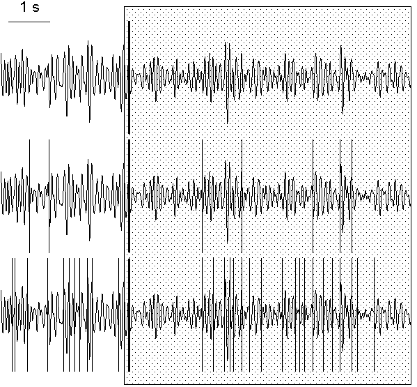
Fig. 7.5. EEG filtered in alpha band (7.5--12.5 Hz) and change-points detected with different false alarm probability
The change-points (vertical lines) were detected in the basic diagnostic
sequence with the following "false alarm" probability sets: at the preliminary
estimation stage (0.2, 0.15, 0.1), (0.6, 0.5, 0.4), (0.8, 0.75, 0.7) for the
subintervals of
L ≥ 100, 50 ≤ L < 100 and 25 ≤ L < 50
correspondingly; at the rejection
stage (0.04, 0.02, 0.01), (0.4, 0.2, 0.1), (0.7, 0.6, 0.5) for the same
subinterval length ranges, correspondingly. For the convinience, the
change-points are shown against the same filtered EEG. Horizontal scale: 1 s.
The "strongest" change-point, which was found as the first one at the
preliminary estimation stage (solid vertical line), can be related to the
subject's reaction to the beginning of presentation of a highlighted image
(the period of presentation is shown by shaded area). The subject (tw09) was
asked to memorize the image.
To solve the problem is especially easy when only one, clearly most prominent change-point must be found in a given interval; this is the task solved in the above discussed work of Deistler et al. (1986) using parametric approach. With our procedure, it is sufficient to determine only the instant of the change-point which will be found the first on the stage of the preliminary estimation. The "false alarm" probability, as one may see from the algorithm, does not affect the order of detection of change-points at this stage. The only serious problem is that the most prominent change-point will be detected first only if it is located not at the periphery of the studied interval.
An example of the detection of single prominent change-point can be seen also in Fig. 7.5. In this figure, the change-point which was found first is shown as a thick line. This change-point corresponds to the beginning of the response of alpha rhythm to the presentation to a subject a luminous picture which he should memorize. The subject's alpha rhythm was slightly suppressed all the time when he saw the picture, nevertheless, it undergone considerable variations both before and during the presentation. The first change-point was found within approximately 150 ms after the beginning of the presentation and indicated the beginning of the period of suppressed alpha activity.
Another economical way of data processing, which leads to the reduction of the number of change-points and enables detection of only those which correspond to long-term transformations of the signal, is the compression (condensation) of the diagnostic sequence. Its simplest form is "thinning out" the data, i.e., the use, instead of a sequence x(t), a sequence x(kt), t=1,2, ... for some fixed k>1. To avoid the loss of information, averaging of data in successive windows can be used instead of "thinning out". The compression of the diagnostic sequence is especially effective in the analysis of the EEG recorded throughout night sleep. The EEG is an excellent indicator of sleep stages, because the electrical activity of the cortex strongly depends on them, but the analysis of sleep EEG is complicated by the huge amount of data to be processed (8 h of sleep means, if EEG is sampled with digitizing rate 100 Hz, 2,880,000 samples for each channel). The compression enables rapid detection of most prominent changes in such a recording (Fig. 7.6).
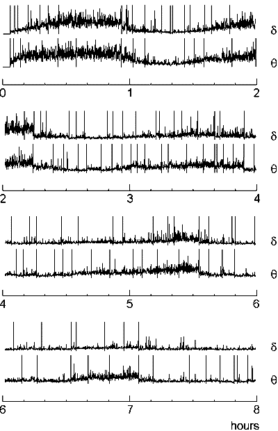
Fig. 7.6. Change-points in sleep EEG: an example of data compressing
EEG was recorded from right occipital electrode (O2) during 8 h of night sleep with sampling rate 400 Hz and downsampled to 20 Hz. After artefact edition the EEG was filtered in 1--4 Hz (delta) and 4--7 Hz (theta) frequency bands, the amplitude values were squared and then averaged in sequential non-overlaping windows (length 5 s, or 100 samples). The resulting sequences are shown (in each pair the upper curve is for theta band and the lower one is for delta) along with the change-points (vertical lines) detected in them.
Change-points themselves say little about brain functioning; further data processing is necessary for the extraction of useful information in the form of various quantitative indices. The most simple approach is comparing the number of change-points per time unit in EEG obtained from different subjects, or from the same subject in different states, or from the same subject's different brain sites (in different electrode locations). It seems to be natural to suggest that the higher is the number of change-points, the more complex is the EEG structure.
However, the number of change-points is not a robust index; it may be sensitive to various factors, even not related to the brain activity. The probability of accepting a statistically justified decision about the presence of a change-point in an interval of a given duration, for instance, depends on the amount of available information, which, in its turn, depends on sampling (digitizing) rate and on the specific features of the process under study (the higher is the frequency of a periodic process, the more information it can carry). Moreover, it must be taken into account that the dynamics of the electrical potential on an EEG electrode can result from superposition of the activity of different systems, or, more precisely, of different "generators", the neuronal networks generating the electrical potential, each network with its own dynamics of the potential. The functional interpretation of a change-point in a signal produced by a single "generator" can be rather clear, but if there is a superposition of potential dynamics from different signal generators, then the interpretation becomes much more complicated. The number of change-points in this case may vary with changes in the ratio of the overall power of the different generators, if they produce signals with different complexity of the segmental structure. For example, an increase of the relative contribution from a generator producing a low structured signal will cause "blurring" the change-points contributed from a generator with highly structured signal, decreasing the total number of statistically detectable change-points; and vice versa. A relatively low number of change-points should be expected also in a signal resulting from superposition of a number of signals with high number of change-points and roughly the same overall power. Nevertheless, we believe that, with caution and with taking into account other indices, the index of the number of change-points can be used in the analysis of the EEG.
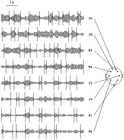
Fig. 7.7. Multi-channel EEG: change-points in alpha activity
The EEG was filtered with bandpass 7.5--12.5 Hz. Change-points (vertical lines) were detected in the basic diagnostic sequence. Subject tw03, eyes closed. Horizontal scale: 1 s.
Variations of the electrical activity across cortical sites can be seen from Fig. 7.7. The overall alpha band power increase from frontal to occipital sites, a pattern usually found in healthy persons. As for change-points, no systematic variations in their number seem to be detectable by visual inspection. Quantitative analysis of this index, however, reveal some regularities. In Fig. 7.8, variations of the number of change-points across subjects are evident. For instance, the number of change-points was especially high for subject tw09 and low in subjects tw07 and tw08 (in the latter case, the alpha rhythm was high but poorly modulated). A certain similarity was found in identical twin pairs (tw07 and tw08 was such a pair), which is in agreement with the other authors' data about the genetic determination of at least some of the EEG characteristics.
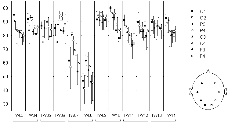
Fig. 7.8. Rate of alpha power change-point occurence in different EEG channels
Genetically identical twins (twin pairs: tw03--tw04, tw05--tw06, etc.). The EEG was recorded in eyes closed condition with 8 electrodes at standard positions (O1, O2, P3, P4, C3, C4, F3, F4). Each EEG channel was filtered with bandpass 7.5--12.5 Hz (alpha). The change-points were detected in the basic diagnostic sequence. Number of change-points in 1 minute EEG (median +-25%; n=3...8 for tw03-tw07; n=10 for tw08-tw14).
The most important finding was the dependence of the number of change-points on the electrode location. In most of the subjects a frontal-occipital gradient was found: the number of change-points was highest in occipital areas (O1 and O2) and lowest in frontal areas (F3 and F4). This dependence did not coincided with the dependence on the electrode location for the EEG pattern and, in particular, for the alpha band power: for example, in tw09 the gradient was almost absent for the change-point number while was well-defined for the alpha band power; his twin brother tw10 had the same gradient for the power and a very clear gradient for the change-point number. Consequently, the gradient of the change-point number hardly was just a reflection of the power gradient, but could be determined by some "structural" features of the alpha activity dynamics, which vary across cortical areas and across subjects.
This view is consistent with a large body of data, obtained with a broad variety of methodical approaches and suggesting the existence of a number of "generators" of alpha activity, which occupy different cortical areas and produce alpha activity with different dynamical characteristics (e.g., Lehmann 1971; Thatcher et al. 1986; Ozaki & Suzuki 1987; Lutzenberger 1997; Florian et al. 1998). Though the structural characteristics of the EEG are still poorly understood, there are strong grounds to believe that they differ for the different "alpha generators" (Basar & Schurmann 1997; Basar et al. 1997; Lutzenberger 1997).
The data presented in Fig. 7.8 were obtained in rest condition with eyes
closed. In the rest condition but with eyes open, the alpha band power
decreased and the pattern of alpha activity substantially
altered, but the number of change-points did not differ significantly for any
electrode location (significance level p>0.05, Wilcoxon matched pairs test).
Our data still not allow to decide whether the lack of significant difference
came from the stability of individual structural characteristics of
EEG alpha activity, or the method was simply not quite sensitive to such
characteristics. A situation may be rather complex: for example, in eyes
open condition the contribution of the high alpha segments to the EEG may be
reduced, then the signal to noise ratio will grow for "finer"
change-points, resulting in the absence of detectable difference in the total number
of change-points. In any case, the data shown in Fig. 7.8 demonstrate that
the index of the number of change-points possesses sensitivity to some EEG
features, since it varies across subjects and brain site.
In EEG signals registered simultaneously from different brain sites (see Fig. 7.7), change-points often appear close in time. A question arises of whether such near-coincidence of change-points could be used in estimating the synchrony of operating of different brain areas (Kaplan et al. 1995; Kaplan et al. 1997a; Kaplan et al. 1997c). This question, in its turn, brings up a number of new methodical issues, which will be discussed in this subsection. Below we will use the terms "coincidence" and "coinciding" instead of "near-coincidence" and "near-coinciding" for short.
For the detection of the change-points which will be used for the estimation of the synchrony, a higher "false alarm" probability can be used. It assures the lower probability of missing a change-point and, therefore, the higher number of change-points detected, making possible more accurate estimation of the level of change-point synchronization. The increase in the number of "false" change-points, in the present context, cannot strongly affect the results of the analysis. The "false" change-points contribute only to the fractions of non-coinciding and randomly coinciding change-points, but do not increase the number of systematically coinciding change-points. The number of randomly coinciding change-points (the noise level) can be easily estimated using the total numbers of change-points in each EEG channel, and thus the estimate of the number of systematically coinciding change-points can be cleared from the randomly coinciding change-points, both "true" and "false". One may see that the estimation of synchronization therefore includes a sort of additional validation of a change-point, which is taken into account only if "confirmed" by the presence of another change-point in a different EEG channel roughly simultaneously with the first one.
The estimation of change-point synchronization is essentially an analysis of synchronization of point processes. Such an analysis was well developed in neuroscience research, mainly in the investigations of impulse activity of single neurons (various methods are described in (Perkel et al. 1967; Gerstein et al. 1978; Gerstein et al. 1985; Palm et al. 1988; Aertsen et al. 1989; Gerstein et al. 1989; Frostig et al. 1990; Pinsky & Rinzel 1995). Surprisingly, this type of analysis has been completely ignored before in the EEG-based research (the only work we know is Guedes de Oliveira & Lopes da Silva 1980); this may be the result of lack of means for the extraction of such EEG "elements" which can be approximated by points.
Fig. 7.9. Illustration for the analysis of change-point synchronization in multichannel EEG
Subject tw03, eyes closed. Each EEG channel was filtered with bandpass 7.5--12.5 Hz (alpha). The change-points were detected in the basic diagnostic sequence. For each change-point in channel O1 a time window (13 samples, or roughly 100 ms, from each side) is positioned. Below the chart the total number of change-points from other channels which fall into the window is shown. Such change-points are considered as coincided with the change-point in O1.
The most simple and, nevertheless, quite effective procedure is the use of some time threshold for the decision about the coincidence: change-points in different channels are considered as coinciding if the time distance between them does not exceed the time threshold. Fig. 7.9 illustrates this approach: each change-point in the first channel (left occipital electrode) is surrounded by a "window" (in this case, by 100 ms to each side from a change-point); all the change-points in other channels are thought to be coinciding if falling into this window. It turned out that these case are not rare, in spite of the fact that some of the change-points were detected in the intervals of continuous change of the signal, which cannot be adequately represented by a single point on a time scale. Moreover, one window most often caught change-points from a number of channels.
On the basis of this procedure, the estimation of synchronization can be made in different ways, such as an estimation of synchrony indices for pairs of channels or a search for most frequent multichannel combinations of coinciding change-points. Details of the algorithm may vary in a wide range: for example, in a search for multichannel combinations it is convenient to use fixed windows placed successively one after another along the EEG recording instead of the windows related to change-points.
The number of pairs or multichannel combinations of coinciding change-points can be used in itself as an index of functional coupling of the corresponding brain areas. This number, however, vary with the number of change-points in each channel. Moreover, it may be "contaminated" by randomly coinciding change-points and therefore, in many cases, not give a good idea of the level of non-random coincidence. To get the "purified" estimate, we may subtract an estimate of the number of randomly coinciding change-points pairs or more complex combinations from the actual number of pairs or combinations. The estimate of the random number can be calculated on the basis of the number and distribution of the change-points in each channel. The "purified" estimate can be then normalized in some way dependent on the specific research aims, for example, by division by the minimal or maximal (across the channels) number of change-points, or by the estimate of standard deviation for the randomly coinciding change-points.
Below we discuss the specific methods of the analysis of change-point
synchronization and results of their application to the processing of real
EEG for the most simple scheme of the analysis, by pairs
of channels, and also a number of more complex schemes.
Analysis of simultaneous coupling of the activity from more than one brain areas by traditional methods is a complex and still poorly elaborated, while more simple form, the pairwise analysis, is broadly used. The most usual indices for functional association between two brain areas are the linear correlation coefficient and coherency estimations computed for a pair of EEG channels. We tried to reproduce some effects which are well established for these indices, using an index of interchannel synchrony based on change-point coincidence.
The index of coincidence (IC) was computed as follows:
ICAB = (NAB - MAB) / (σAB),
where NAB is the empirical number of coinciding change-points in channels A and B, MAB and σAB are the estimates of the mathematical expectation and the standard deviation of the number of coinciding change-points correspondingly under condition that the coincidence is random (i.e., the change-points in different channels are independent of one another).
We can estimate MAB as follows. Let us define the point process corresponding to the sequence of the change-points for a given channel: the process at instant t is equal to 1 if there exists the change-point at the moment t, and is equal to 0 otherwise. We suppose that the point processes are the sequences of identically distributed random variables with the probability of "success" PA and PB respectively. We say that the change-points in channels A and B coincide, if |tA - tB| ≤ τ, where tA and tB are the change-point moments, τ is the time threshold of the synchronization.
Assume that the point processes corresponding to the channnels A and B are independent, and the length τ of the "window" is such that it is improbable to see more than one change-point at the same "window". Under these conditions the probability of simultaneous change-points in both channels at the instant i is equal to PAB = (2τ + 1)PAPB and the mathematical expectation of the number of coinciding change-points (under the condition that τ << N, where N is the length of the EEG) is equal to NPAB.
Assume that there are NA change-points at channel A and NB change-points -- at channel B. Then the estimates for PA and PB are equal to NA/N and NB/N correspondingly. Therefore, we have
MAB = NPAB = N (2τ + 1)(NA/N)(NB/N) = (2τ + 1)NANB/N
Now let us estimate the standard deviation of the number of the coinciding
change-points under the hypothesis that the corresponding point processes are
independent. Suppose that the point process corresponding to the coinciding
change-points is the sequence of independent and identically distributed
random variables with the probability of "success" PAB. Then
we have for the standard deviation of this point process
 .
Therefore, the estimate of the
standard deviation of the number of the coinciding change-points if the
hypothesis of independence is true has the form
.
Therefore, the estimate of the
standard deviation of the number of the coinciding change-points if the
hypothesis of independence is true has the form
 .
.
One can easily see that the index of coincidence, in average, tends to zero in the case of no coupling between the change-points and takes positive values when there is coupling or, more exactly, if the change-points in different channels have a tendency to appear closer to each other than the time threshold of coincidence.

Fig. 7.10. Brain topography of alpha change-point coincidence
Each schematic map shows the level of the index of alpha power change-point coincidence (see text) for pairs composed of one electrode (small black circle) and each of the others (large circles with shading density representing the level of index; see legend at the top). Averaged data from 12 subjects, eyes closed. EEG was filtered with bandpass 7.5--12.5 Hz (alpha). The change-points were detected in the basic diagnostic sequence. The time threshold of coincidence (time "window") 13 samples (approximately 100 ms). (From Shishkin & Kaplan, in press.)
Fig. 7.10 presents of the indices of coincidence for change-points in alpha band power, computed for all pairs of eight EEG channels. The values of the indices were averaged across subjects. The index of coincidence was apparently above zero for most of the electrode pairs, i.e., the frequency of coincidence of change-points was higher than the random level. A clear dependence of the index of coincidence on topographical factors is evident: first, the higher is the interelectrode distance, the higher is the index; secondly, with the same interelectrode distance, the index is higher for more anterior pairs of electrodes. These effects are in full agreement with the data obtained for the synchronization in EEG alpha band by different researchers using correlation and coherency analysis. Our index, however, is based on completely different principles, and the similarity of the results indicates that the different types of signal coupling, estimated by such different indices, represent the different sides of the total phenomenon of the dynamical coupling of electrical potentials produced by different brain systems (Shishkin & Kaplan, in press).
Effects of the topographical factors were then studied in more detail. The same data were treated as 294 EEG epochs of 14 s duration instead of group average. The mean number of alpha power change-points in such epoch was about 20 per channel. A linear regression analysis made across all the pairs of electrodes separately for each of the epochs confirmed the dependence of the index of coincidence on the interelectrode distance and on the position of electrodes on the anterior-posterior axis. In spite of great variability of the EEG and the difficulty to obtain stable estimations on such short epochs, the regression coefficient was negative for the interelectrode distance almost in all the epochs (293 of 294), and positive for the position on the anterior-posterior axis still in a vast majority of the epochs (277 of 294) (Shishkin & Kaplan, in press). This stability of the results is remarkable, especially considering a great intra- and inter-individual variability of alpha activity patterns in our data. Note that 14 s is usually too short interval for stable estimating of most of the EEG parameters. Thus, the results showed a good performance of our method of estimating interchannel synchrony.
The index of change-point coincidence was also found to be sensitive to the condition of open/closed eyes and the interindividual differences in state anxiety, which are other factors influencing the alpha activity. The fact of much stronger alpha rhythm in most of persons when their eyes are closed, comparative to eyes open, is well known from the first EEG studies. More complicated are the relation of the alpha rhythm to the level of anxiety, one of the most important components of the emotional domain which manifests itself in feelings of worry, insecurity, causeless fear, etc.; in general, alpha activity and anxiety are related inversely.
To study the difference between closed and open eyes states, we used a standard experimental scheme: the EEG was registered in both states, the indices were calculated for each EEG recording and averaged for each subject, and then the data were compared statistically (by nonparametric paired Wilcoxon test) for the two states. A state was determined by one of two very simple instructions to a subject: to sit calm and relaxed with eyes open or to sit calm and relaxed with eyes closed. The indices computed for the EEG obtained in the closed eyes condition were also used in the second type of analysis, namely for the estimation of the relation between interindividual variations of the change-point synchronization and the level of anxiety. Two types of anxiety was estimated quantitatively by the scales of standard Spielberger questionnaire. The first one was state anxiety which corresponds to the subject's anxiety at the moment of experiment; the second one was trait anxiety, a personality characteristic describing the general susceptibility to anxiety. A correlation coefficient (Spearman's R, which is a rank analogue of Pearson correlation coefficient) was computed between each of the two anxiety indices and the indices of coincidence for alpha power change-points for each pair of EEG electrodes. Correlation was not significant for the trait anxiety (significance level p>0.1 for all electrode pairs) but significant between the state anxiety and the indices of coincidence for 10 of 28 electrode pairs (p<0.05). The results were presented in a form of maps showing the pairs of electrodes significantly related to the factors of open/closed eyes (Fig. 7.11) and state anxiety (Fig. 7.12).

Fig. 7.11. Pairs of EEG electrodes where alpha change-point coincidence differed in eyes closed and eyes open conditions
Lines connecting pairs of electrode positions represent significant difference for those pairs (Wilcoxon matched pairs test, n=12): thick, p<0.05; thin, p<0.1; filled, index of coincidence is higher with eyes closed; blank, index of coincidence is higher with eyes open. (From Shishkin & Kaplan, in press.)
The map of open/closed eyes difference (Fig. 7.11) reveals that the higher level of alpha power change-point synchronization with eyes closed was specific for anterior regions, while with eyes open it was higher in pairs including one of the occipital electrodes. The same tendencies were observed for all anterior pairs and all pairs including an occipital electrode even in the cases of non-significant difference, except for two pairs with the most low difference.
As we noted above, the number of the change-points in eyes open and eyes closed did not differ significantly, thus it could not be responsible for the clear differences of the indices of change-point coincidence. Since the differences in the overall alpha band power between eyes closed and open conditions are high (especially in posterior regions), their influence on the results of change-point detection cannot be fully excluded; however, they alone are unable to explain the topography of the effect, and the presence of actual difference in the degree of association between the signal structure in different channels was most probable. The results, while still not elucidating any brain mechanisms, demonstrate the usefulness of our approach in the study of the generation of alpha activity.

Fig. 7.12. Pairs of EEG electrodes where alpha change-point coincidence correlated with state anxiety
EEG was recorded in eyes closed condition. Lines connecting pairs of electrode positions represent significant correlation with anxiety index for those pairs (Spearman rank order correlation, n=12, p<0.05).
The electrode pairs with significant correlation between the index of coincidence and the state anxiety are shown in Fig. 7.12. All the significant correlation coefficients were positive, i.e., the subjects with highest anxiety had the highest change-point synchronization, and vice versa. It should be noted that the subjects with higher state anxiety also had lower overall alpha band power, and in this way this inter-individual effect was opposite to intra-individual effect of open/closed eyes factor -- in the latter case, the index of coincidence was increased when alpha activity was also the highest (with eyes closed). Thus, in the two different types of analysis (inter- and intraindividual) the tendencies of the relation of the overall power and the synchronization of change-points in power of the same band appeared to be opposite, giving a strong evidence that the sensitivity of our index to variations of different psychophysiological variables was not just a derivative of the changes in mean level of EEG alpha band power.
The relationship between the index of coincidence and the state anxiety had a rather specific topographic feature: significant correlation was found mainly for interhemispheric electrode pairs, i.e., the pairs including electrodes located over the left and right hemispheres of the cortex. It is widely accepted that the interhemispheric interactions is important for the emotional domain and for such its component as the anxiety level. Our data are in agreement with this view, suggesting that the interhemispheric interactions significant for the anxiety level may manifest themselves also in the segmentary organization of the EEG alpha activity. These data, like the open/closed eyes effects discussed above, demonstrate the sensitivity of our index to the human brain state.
However, it must be kept in mind that the change-point synchronization is even more complex function of various factors than the number of change-points (discussed in subsection 7.5.4). For example, suggest that the electrical signal in each of two EEG channels is composed of two different alpha band components, one of which is presented equally in both channels and therefore "produces" synchronized change-points. The superposition of the second component with the first one leads to decreasing the probability of detecting the first component's change-points (in this situation, the second component is a sort of noise). In such a case, the variations in the estimated synchrony can be accounted not only for the variations of the first component, but also for the variations in its ratio with the second component. Moreover, the increase of the second component may cause the decrease in the estimated change-point synchronization between two electrical signals not only if it carry its own change-points and is present only in one channel, but also in the case when it is present in both channels (the two resulting signals thus are synchronous!) -- if it has no own change-points at all.
Unfortunately, the other methods of estimating the coupling of different
signals, which are used in EEG analysis for the investigation of functional
relationships between brain sites and structures (such as correlation or
coherency analysis), are subjected to the same problems. Our approach,
however, has his own value, since the change-point coupling is an index
of features of intersignal association different from what is monitored by
correlation, coherency or other known characteristics.
The change-points, as it can be seen in Fig. 7.9, often appear near-simultaneously in more than one channel. It is naturally to treat the change-points appearing close in time in a number of EEG channels as a single complex. We will call it a change-point synchrocomplex, or simply synchrocomplex. Since the different EEG channels represent the activity from different cortical areas, which lies under the corresponding electrodes, the synchrocomplex represents the topography of sharp transformations of electric activity, which occur in these areas in synchrony or almost in synchrony and probably reflect the functional connectiveness of these areas.
The spatial configuration of the functionally connected areas may vary dramatically within even short time intervals, and this dynamics may manifest itself in change-point synchrocomplexes. The configuration of a change-point synchrocomplex (defined as the set of EEG channels containing the change-points which constitute a synchrocomplex) therefore can be an informative characteristic of the current brain state, and a set of such configurations found in a given EEG can represent the variety of brain states during the interval of the EEG recording. It is evident that such a set of configurations cannot be estimated only on the basis of the information provided by the pairwise analysis described above: the same mean values of the synchrony indices for the pairs of channels can be observed in the cases of absolutely different sets of the configurations of change-point synchrocomplexes. If the distances between neighbouring electrodes are roughly equal, the number of change-points participating in a synchrocomplex, which we call the order of synchrocomplex, provides an estimate of the total cortical area were the activity changes simultaneously.
An accurate definition of a change-point synchrocomplex must include a certain time threshold for change-points to be included, in a form of a short time window covering both the earliest and the latest change-points of the complex, or in a form of the maximal allowed time distance between successive change-points. In practice, a more crude way to define synchrocomplexes can be used for simplicity, especially if the probabilities of certain configurations should be computed: the analysed EEG recording is divided into fixed windows of equal lenght, and each window is characterized by the presence or absence of a change-point in each channel. The length of the "window" is chosen so that it covers no more than one change-point from each channel, and yet the cases when the border between two windows separate two apparently close (in time) change-points from different channels are not very frequent.
The probability of simultaneous appearing by chance of change-points in different channels falls very quickly with the increase of their number, so that, in practice, all the "higher order" synchrocomplexes can be considered as "real", showing some actual degree of connectiveness between EEG channels. For simplicity, we may consider only the number of synchrocomplexes of a given configuration as the main index, keeping in mind that the "low order" synchrocomplexes may result from casual coinciding of change-points and that they require special caution in the interpretation of results. The configurations of the synchrocomplexes can be ranged in accordance with their rate of occurence, and then only the most frequently found configurations are analysed.
The analysis of change-point synchrocomplexes can be illustrated more clearly if the spatial dimensionality of the EEG is reduced to one dimension by using the electrodes placed along one line. We applied the electrodes with equal distances between them as a "chain" from the forehead to the occipital (over the standard positions O2, P4, C4, F4, and between them). By this way we could not, of course, get the entire spatial picture of the cortical potentials, but, in return, gained in spatial resolution with relatively low number of electrodes (specifically, 16 electrodes).
Each of 10 artefact-free EEG recordings (1 minute, 7680 samples; eyes closed, resting) was subjected to the change-point detection and then was broken into 590 successive "windows" of 13 samples (about 100 ms) length. In 47.3% of "windows" no change-point was found in any of the channels. In 9.9% of "windows" a change-point was found only in one channel. The low number of such "singular" change-points can be attributed primarily to the dense positioning of the electrodes: the electric potential dynamics at close points on the scalp is very similar because of high functional connectivity of close cortical areas and because of volume conduction effects. The coincidence of change-points at different electrodes, if the spaces between them are not too large, is, however, very usual in more general situation (see, for example, Fig. 7.9).
The presence or absence of a change-point in a channel of a certain "window" can be denoted as 0 or 1, respectively. Then each window will be denoted by a combination of 16 binary digits, each digit corresponding to a channel. The combination describes the configuration of a synchrocomplex in this "window", if change-points are found in two or more channels simultaneously. A possible number of such combinations is rather high (216=65536) and it could not be convenient to analyse the rate of occurrence of each combination separately. In 10 minutes of our EEG recording (5900 "windows"), however, only 805 of the combinations were found, of which 788 described the configurations of synchrocomplexes, 16 -- "windows" with a change-point in only one channel and 1 -- no change-points in a "window" at all. The 788 configurations was still a large set, and it was important to see whether some of them were very rare and resulted from random coincidence of the change-points, or was unseparable from those "random" configurations.
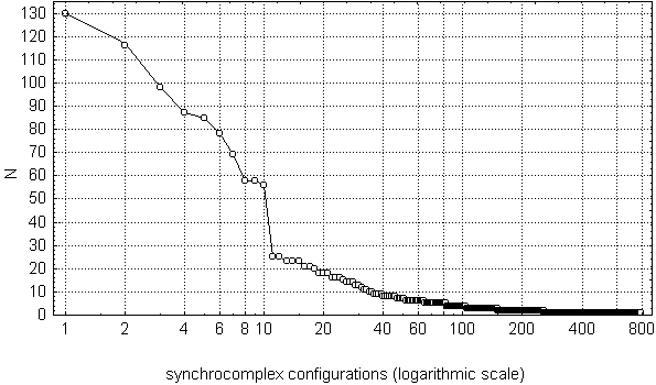
Fig. 7.13. Variation row of synchrocomplex configurations
Horizontal axis (logarithmic scale) represents synchrocomplex configurations
in occurrence rate decreasing order (each point on the axis corresponds to a
single configurations); vertical axes represents their occurrence rate (as
the total number of the synchrocomplexes with the given
configuration).
Subject EGL. 10 one-minute EEGs were recorded in eyes closing, resting condition.
Electrodes were placed with equal spaces between them along
anterior-posterior axis at right side of the head. Their
numbers started from the occipital. EEG was filtered with bandpass
7.5--12.5 Hz (alpha), the change-points detected in the basic diagnostic
sequence. Synchrocomplex configuration was defined by the
set of channels in which the coinciding change-points were found (for more
details see text).
As it can be seen from Fig. 7.13, most of the configurations were found very rarely: from 2 to 3 cases -- 152 configurations, 1 case -- 532 (!). Only 35 configurations were found more than 10 times (more rare than one per minute in average), but the total number of "windows" with these configurations was 1256 (21.3% of the total number of the "windows"), i.e., almost equal to the number of the other synchrocomplex configurations (1265, or 21.4%). Most prominent at the Fig. 7.13 are 10 most frequent configurations, each of which was found in no less than 56 "windows". Taken together they occupied about 1/7 of the total number of "windows", or 26.9% of those "windows" were at least one change-point was found.
Fig. 7.14. Most frequent configurations of synchrocomplexes
Synchrocomplex configurations (change-points in alpha band power) found at least 10 times in 10 one-minute EEG recordings (same EEGs as in Fig. 7.13). Black circles: electrodes where change-points were detected. Electrode positions are shown in the right. N -- number of observations, "!" -- configurations with highest rate of change-point occurence.
Thus, a half of the synchrocomplexes found in these EEGs had one of 35 most frequent configurations, which is only 1/1872 of all possible configurations. These most frequent configurations are given in Fig. 7.14, and the top frequent 10 -- also in Fig. 7.15. Due to the linear scheme of electrode montage the linear notation used for synchrocomplex configurations in these tables give a picturial view of real spatial relations of the areas with synchronous changes of electric potential dynamics in alpha band on the head surface.
Fig. 7.15.
A remarkable characteristic of 30 of the 35 most frequent synchrocomplex configurations (given in Fig. 7.14) is their unbroken structure, i.e., all the channels with change-points in them were in succession. The five configurations with breaks were relatively infrequent (the most frequent of them, with change-points in channels 12,14,15 and 16, was found only 16 times during the 10 minutes of the EEG registration); in all these cases the break involved only one channel and the outer borders of these configurations exactly matched the outlines of the most frequently found (58 or more) synchrocomplexes. It is likely that the broken configurations were caused by artificial deviation from the frequent ones with a miss of a change-point. Thus, the areas under our electrode chain with simultaneously observed change-points in alpha band power typically were continuous (unbroken). This is an example of a fact which can be determined only with the multichannel, but not pairwise, analysis.
Another interesting spatial characteristic of these data was the higher rate of occurence of the higher order (i.e., more extended) synchrocomplexes in the anterior relative to posterior areas of the head. This phenomenon probably reflected the same intrinsic spatial features of the alpha activity as the higher level of change-point synchronization in anterior areas determined by the pairwise analysis.
The low percentage of the synchrocomplexes with broken configurations showed that the casual miss of a change-point only slightly affected the results. There were also another characteristic feature of the frequent configurations which could be observed only in the case of low influence of the missing change-points: the frequently found synchrocomplexes of the same or similar orders, as it can be seen in Table 7.2, did not overlapped. The method we used, though a very simplified, thus demonstrated a rather high ability to study the change-point synchrocomplexes.
We are now only in the beginning of the practical use of the EEG change-point
synchrocomplex analysis, and it is too early to draw more certain conclusions
on the basis of these data. The results described in this subsection should
be considered not from the point of view of revealing certain
physiological mechanisms but rather as an illustration of the potential of the
multichannel approach to change-point synchronization analysis. In the next
subsection we will discuss the general characteristics of the change-point
syncronization methodology and give the outlines of some other
ways of its developing.
It is necessary to note that a change-point detection method which we applied to a real EEG signal was developed on the basis of the piecewise stationarity model of the signal. The performance of the method in the cases of gradual transitions from one segment to another, which are often observed in the EEG recordings, could not be completely adequate. But how much this discrepancy between the real signal and the model influenced the results?
Indeed, when the transitions from one segment to another were gradual, they
usually were broken by the estimated change-point approximately in the middle,
so that they were partly included into the estimated adjacent segments
(Fig. 7.4, 7.7, 7.9). The other known methods of the EEG segmentation are
also subject to this shortcoming, in part because many of them also utilize
the piecewise stationarity model (Barlow 1985). In our work, however, the
transitions themselves were usually well detected even if they were
substantially long (see Fig. 7.4, 7.7, 7.9), making possible an effective
analysis based on the describing the transitions as the points on time axis.
Particularly, the interchannel synchronization of the EEG change-points was
considerably above the stochastic level, excepting the cases of the
highest interelectrode distance. It must be kept in mind, however, that in
the cases of higher deviations from the piecewise stationarity model than
those observed in our data the signal may lose the structure available for
the analysis of any kind, and it will be just senseless to characterize it
with change-points.
One of the problems related to the nonstationarity may appear to be
fundamentally unsolvable in the application of the change-point methodology
to highly nonstationary signals like the EEG. In the calculation of any
averaged estimate of synchronization between signals, not only the
traditional correlation/coherency but also change-point based, the
possibility of the nonstationarity of synchronization level itself is ignored.
No evidence exists that at the different time intervals the coupling between
signals (or signal components) cannot possess different mean values.
More generally, any characteristic estimated for a large time interval, even
if segmentation approach is applied, can be a subject to this problem. The
same task as discussed above in the formulation of the problem of EEG
segmentation appears here: any value computed for some time interval may
be quite far from the real levels of the estimated characteristic at any part
of this interval. This problem, in a special case of estimating the
probabilities of transitions between different classes of EEG stationary
segments, was noted in the paper of Jansen and Cheng (Jansen & Cheng 1988). It seems to be
reasonable to keep always in mind that if the signal of weakly understood
nature is nonstationary (like the EEG), any of its characteristic may appear
to be nonstationary; this means that any averaged estimates of such
signals must be used with caution.
The revealing of the instants of changes in the EEG or other complex signal makes more precise the routine statistical analysis, which usually require stationarity of the signal interval in question. We will not consider here the possibilities of the EEG analysis being opened by viewing it as a sequence of stationary intervals, since they were extensively discussed by other authors in the works related to the EEG segmentation (e.g., Bodenstein & Praetorius 1977; Sanderson et al. 1980; Creutzfeldt et al. 1985; Barlow 1985; Jansen & Cheng 1988; Cerutti et al. 1996; Pardey et al. 1996). In our work, probably for the first time, the emphasis was made on the other aspects of the utilizing the information about the signal structure given by the time instants of changes.
The data presented in this Chapter demonstrate that the effective detection of the change-points opens the way for a number of new methods of the analysis of complex signals such as the EEG. First, the segmentary time structure of the signal or (if the signal is composed of a number of components with more or less independent dynamics) its components can be accurately described. Secondly, if these descriptions are obtained for two or more simultaneously recorded signals or for the components of the same signal, their temporal relations can be estimated. These approaches are empirical in their essence and have no explicit mathematical justification, at least now, but at the current stage of the studies of the EEG structural characteristics they seem to be quite acceptable, because of the lack of the understanding of the EEG nature and the weak elaboration of more strict methodology of its structural analysis.
The separate detection of changes in different frequency bands and with different time scales was already used by other researchers (Deistler et al. 1986; Ferber 1987). In our work this was done with a more broad range of signal types, covering a substantial portion of the variety of patterns occurring in the EEG studies. It turned out that the detection algorithm described in this book easily worked with all of them, requiring only little "manual" efforts for tuning its parameters, or allowing unsupervised automatic data processing (Fig. 7.2-7.4, 7.6).
One of the possibilities of signal analysis offered by the change-point
detection, namely the statistical estimation of the temporal relationship
between the segmentary structures of different signals and of
different components of the same complex signal, was not employed before our
works at all. This is why we will focus our attention on it here.
The realization of this possibility was supported by the ability of the method described in this book to detect, in unsupervised regime, high number of change-points with high accuracy. This makes possible describing the structure of a piecewise stationary process by a point process, comprised of the change-point instants. We are based on the assumption that the change-point moments correspond to especially informative "events" of the brain systems dynamics, namely to their "switches" from one microstate to another. In this case the simultaneity of the occurrence of the change-points generated by different systems gives an evidence of some kind of connectivity in their functioning. Detailed information about signal generation, as well as constructing the model of the signal, is not required, only some concept of the functionally significant components composing the signal is helpful. Essentially reducing the signal to the series of discrete events greatly simplify the consequent analysis, particularly the analysis of temporal relations between a high number of simultaneously registered signals, still expecting to keep the most relevant information which is hidden in the signal structure.
We proposed this approach in 1995 (Kaplan et al. 1995) and latter developed it in a number of publications (Kaplan et al. 1997a,c, 1998; Kaplan 1998, 1999; Shishkin & Kaplan, in press). A similar method was suggested in 1997 by Hofmann and Spreng (Hofmann & Spreng 1997); this method was based on counting the number of coinciding segment boundaries, which were determined using the clasterization of fixed epochs. The method of Hofmann and Spreng seems to be effective in certain situations, but less sensitive in a general case, since the segment boundaries are established with low temporal resolution (0.64 s). (See also the discussion of the "fixed-interval" segmentation in this Chapter, Subsection 7.3.1.)
A promising approach to use the information about the temporal relationship between quasistationary segments in electrical signals registered from various brain structures was suggested by Wendling et al. (1996) and further developed by Wu and Gotman (1998). This approach is pointed at the revealing the sequencies of electrical activity patterns, recurring in exact order and related to the development of epileptic activity. Unfortunately, in most cases normal EEG has less determined features than EEG associated with epileptic seizures, so this method can hardly be adopted for more general purposes.
Creutzfeldt et al. (1985) and Gath et al. (1991) developed their segmentation algorithms in such a way that they were sensitive to such changes which occur simultaneously in different EEG channels. This can be also considered as an example of revealing the structural temporal relationship between different signals, though the authors made no emphasis on this property of their methods and were aimed only at increasing the reliability of the segmentation by a kind of reciprocal "verifying" the change-points in different channels by each other.
Although many other researchers considered the synchronization of the onset and stop of physiological activity at spatially different sites as important sign of the functional relationship (e.g., Andersen et al. 1966), they did not employ special statistical techniques for the justification of the synchronization.
In addition to the change-points, there are some other types of significant events in the EEG which can be reduced to the points on the time scale, for example, single waveforms (especially sharp "spikes") or groups of waves. Some specific patterns characteristic for epilepsy are especially short-term and therefore can be very adequately presented as time points. Their synchronization in the multichannel EEG were indeed studied similarly to the way described above, but only in one work (Guedes de Oliveira & Lopes da Silva 1980).
The analysis of point processes syncronization was elaborated in detail as an application to the problem of estimating the functional connectivity between single neurons. This problem is solved on the basis of assessing the temporal relationship between the sequences of electric impulses (spikes) generated by the neurons (Perkel et al. 1967; Gerstein et al. 1978; Gerstein et al. 1985; Palm et al. 1988; Aertsen et al. 1989; Gerstein et al. 1989; Frostig et al. 1990; Pinsky & Rinzel 1995). The nature of the point processes in the case of the EEG change-points is substantially different: the points correspond not to clearly defined events such as neuronal spikes but to statistically detected instants of the transformations of the signal components. Nevertheless, the statistical characteristics of the both types of point processes do not much differ, so the methodology of the analysis of neuronal spikes synchronization can be adopted in the studies of the multichannel EEG change-point synchronization. Such methodology also was applied in the EEG-related work cited above (Guedes de Oliveira & Lopes da Silva 1980).
The most considerable difference between the change-points and such phenomena as neuronal impulses or epileptic spikes is much more variable nature of the change-points in the EEG: the EEG change-points may result from a wide range of neuronal activity transformations. This circumstance should be always considered in interpretation of the results obtained using the change-point methodology. But it is not a crucial shortcoming, since the traditional methods successfully applied to the EEG analysis, such as correlative or coherency analysis, also cannot differentiate the elements of the signal (in this case, the subsequent amplitude values) related to different processes on the physiological level. If in the further development of the methodology some special methods of selection of the events or components of the same physiological nature will be introduced, they could probably make the outcome of the analysis more sound and sensible.
The temporal relationship between the change-points in different channels can be described most completely using the information about their relative time of occurrence. If, for example, a change-point in channel A often precedes a change-pont in channel B with relatively constant delay, this may be considered as an evidence for a certain functional relationship between the brain areas monitored by these channels; the operational "switches" reflected in A probably cause those reflected in B. In practice, however, the high variability of the EEG makes such type of analysis rather complicated, since special precautions must be taken against systematic bias of instant estimates which may be probably caused by specific EEG patterns, and relatively large amount of data are required to get stable estimates. Therefore, we still restrict our work to more rough approach to study of the synchronization between point processes, which ignores the exact time delays between the near coinciding change-points and only takes into account the fact of the near coincidence itself, defined by a certain time threshold.
Our experimental results showed that the near coincidence of the
change-points in pairs of the EEG channels occurs, in general, much more
often than one may expect in the absence of relationship between the
cortical areas from which the electrical activity is derived. Moreover,
the index characterizing the non-stochastic level of the alpha band
change-point near coincidence appeared to be sensitive to the difference
between eyes closed and opened states (Fig. 7.11) and to the
individual level of anxiety (Fig. 7.12).
Since the EEG signal is a mixture of relatively independent components
differentiated by their frequencies, the extraction of these components and
separate detection of their change-points leads
to representing the EEG as an assembly of different point processes. Their
interrelationship (the interfrequency consistency) can be estimated using the
same techniques as in the case of interchannel analysis. The level of
change-point coincidence in many of the pairs of the standard EEG frequency
bands, both in the cases when they were taken from the same EEG channel or
from different channels, also exceeded the stochastic level
(Kaplan et al. 1998). In the general case, one may
speak about estimating the structural temporal relationship between a
number of components extracted, by some means, from one or from a number of
signals, i.e., estimating the intersignal and/or intercomponent (including
their combinations) structural relationship. In the case of different
frequency components, it is worth to note that there is no restrictions for
the relations between frequency bands, because the analysis is not associated
with the phase relation as the usual techniques.
When a number of signals are recorded simultaneously, as in the case of multichannel EEG, the pairwise analysis of the coupling between different signals (channels) gives only partial description of the inherent relationships. Assuming that different brain areas may co-operate in different combinations within the interval of observation, one may expect that the simultaneous change-points will appear in different combinations over the channels, some of which will be found especially often. For example, the change-points may often occur near-simultaneously as a pair in channels A and B or as a triplet in channels A, B and C, but not as a pair in channels B and C (without a simultaneous change-point in A). It is evident that the pairwise analysis is unable to reveal this pattern in detail.
The frequently appearing combinations, assumed to indicate the temporally established groups of co-operating brain areas, can be estimated, roughly, just by the number of the observed "synchrocomplexes" (as demonstrated above; Fig. 7.14 and 7.15), or, more strictly, using more sophisticated techniques already developed extensively in the analysis of single neuron spike trains which is used for the search for so-called "neuronal assemblies" (Gerstein et al. 1978; Gerstein et al. 1989; Frostig et al. 1990; Martignon et al. 1995; Strangman 1997; Lindsey 1997). The reduction of the initial signal to a point process makes the description of the mutual connectivity among more than two signals more easy than with the computation of mutual correlation or coherency.
As evidenced by the foregoing, the analysis utilizing the change-point near-coincidence provides, potentially, various opportunities for the analysis of coupling between two or more signals or components of a polycomponent signal. Though many of those opportunities are still not realized in practice, the first experimental results obtained with the application of this approach to the human EEG, have showed the sensitivity of the indices based on it, and therefore give promise of further success in its practical development.
Finally, it should be said that estimating of coupling between two or more
processes by the frequency of the change-point near coincidence is basically
not a new approach. The coincidence of the time instants of considerable
changes is taken into account not only in the brain research but also in many
scientific fields, in application to a huge variety of processes going in
nature and in society; it is a commonly considered sign of the relationship
between the observed processes even in everyday human practice. In our work,
we have merely combined this approach with the quantitative statistical
method of estimating the instances of changes. We hope that some of the
ways of the quantitative estimation of change-point synchronization developed
in our work could appear to be useful not only in the analysis of the human
brain electrical activity.
Unless in many other approaches to the analysis of different signal coupling,
the information entering the analysis of synchronization in our approach is
explicitly represented in the form of elementary,
instantaneous events (the change-points). Therefore, the following new ways of the
developing the methodology are opened. One may characterize those events
by certain features, such as relative change of the monitored index (e.g.,
the ratio of spectral power in a certain band computed for the
adjacent segments), the type of EEG pattern forming the background against
which the change-point was found, etc., and then preselect the change-points
according to those features before the analysis
of synchronization. On the other hand, each of the frequently found
synchrocomplex configurations can be separately characterized by the features
of their background. Both ways of the analysis may reveal some relations
between the background activity and the instants of its change, and the former
one also provide the means of improving the quality of the analysis by
rejecting less reliable change-points (e.g., too "weak" or found against
too "noisy" background).
Another promising area of the studies of EEG structure based on the reduction of this signal to the change-point sequences is the analysis of the dependence of instances of change and change-point coupling on the time instances of repetitive "external" events, such as presentation of a stimulus to a subject or his rare and rapid movements (e.g., pressing a response button). The time instants of such events can be determined precisely, and therefore they are widely used as time markers for the analysis of the brain activity which may be in some way related to them (the so-called event-related potentials, event-related desynchronization/synchronization, etc.). The disturbing of the brain activity following these events, however, means that in the studied time interval some rapid changes occur (see Fig. 7.5 for an example of strong event-related change-point); consequently, the common linear indices are not well suited for such intervals, and the change-point based analysis seems to be a rational alternative to them.
The lack of the adaptability of the available change-point detection methods
to different time scales and the lack of attention to the change-points
caused by its concentration on the segments prevented the realization of this
alternative. Only in one work the change-point detection was used for the
detection of an "internal" event, the brain activity transformation
following, after a certain time delay, an "external" event, the
administration of a drug (Deistler et al. 1986), and also only in one
work the relationship between the change-points and the external stimuli was
studied (Skrylev 1984). The techniques for the estimation of the changes in
the probability of the point event, as well as of two near-coinciding
events, in the vicinity of a stimulus are, again, developed in the analysis of
neuronal spike trains (Palm et al. 1988; Aertsen et al. 1989; Gerstein et al. 1989; Frostig et al. 1990; Lindsey 1997; Awiszus 1997).
They provide effective means, in particular, for the identification of fast
modulation of synchrony, whereas the analysis of event-related coherency
(e.g., Florian et al. 1998) is restricted by the low temporal resolution of
coherency estimating. At present, we are only in the beginning of application
of those techniques to the EEG change-points.
The most complete understanding of the coupling between nonstationary signals of EEG type can be probably achieved only by the integrated application of different approaches. We found that the basic "topographic" regularities known for correlation and coherency (the dependence of a synchrony index on the interelectrode distance and on the electrode position on the anterior-posterior axis) are well reproduced for the alpha band change-point coincidence index (Fig. 7.10). This on no account can be considered as an evidence for the identity of those indices, because the coincidence of change-points is related to a special type of signal coupling, the structural synchronization, which completely ignores the level of signal synchronization in the intervals between the coinciding change-points. It can be noted, without going into details, that one may expect different relative levels of the linear phase relationship estimates (such as product-moment correlation or coherency) and the change-point synchronization indices when the nature of the signal coupling is different. Hence the use of correlation/coherency estimates in parallel with change-point analysis seems to be quite rational.
More close integration of change-point analysis with the traditional
statistic methods may also be advantageous. For instance, the
"off-change-point" component of the correlation coefficient,
representing the association between two signals not related to their
segmentary structure, can be estimated by calculating the correlation
coefficient only on the intervals without change-points in
both channels and then averaging the obtained values, taking into account
the lengths of the intervals as the weights. Conversely, a correlation
index may characterize the segmentary structure rather than
"off-change-point" component, but, unless the mere change-point
synchronization indices, incorporate the values of the characteristic in
question (e.g., amplitude or power in the given frequency band) computed
for the segments. It can be computed in a following manner: the mean
value of the analysed characteristic is computed in each signal channel for
each time interval between any neighbouring change-points, with no respect
in which channel they were found; this will result in one sequence of means
per channel, characterizing the dynamics of the signal; then it only
remains to compute the correlation coefficient between the sequences
corresponding to different channels.
The method of electroencephalography, or registering the brain electrical activity from the head skin surface, is now the most feasible way to non-invasive study of the brain processes underlying mental activity. The EEG is also an effective tool for brain disease and traumatic lesion diagnostics.
Since the EEG is a very complex signal, a great variety of mathematical methods was applied to it in attempt to extract more information concerning the brain functioning. Most of those methods, however, can provide reliable results only if the inherent "biological" properties of this signal, and especially its high nonstationarity, are taken into account.
The critical review in the beginning of this Chapter shows that even the methods suggested by various authors for treating the EEG as a nonstationary process, especially the parametric methods, are often not well suited for this signal, because they possess an internal contradiction of constructing models without considering the nonstationarity of the intervals to which the model is fitted.
This is why the nonparametric approach to the nonstationary processes suggested and developed by Brodsky and Darkhovsky appeared to be a valuable tool for the investigation of brain functioning on the basis of EEG analysis. The results of the application of change-point analysis to the human EEG described in this Chapter demonstrated the relationship between the piecewise stationary structure of this signal and the brain functioning. The segmentary structure of the electrical activity from different brain sites was shown to be considerably synchronized, and the degree of synchronization appeared to be dependent on various factors of brain activity. Thus, a new phenomenon of the "operational synchrony" was described (Kaplan et al. 1995; Kaplan et al. 1997a; Kaplan et al. 1997c).
From the methodological point of view, effective detection of the change-points on the basis of nonparametric approach by Brodsky and Darkhovsky opened a way for the development of a specific analysis of synchronization between signals, based on the methods of estimation the coupling between point processes (Kaplan et al. 1995).
The experimental evidence described in this Chapter also makes possible a novel approach to the understanding of the basic problems of brain multivariability.
Even now, in the end of the XXth century, when the artificial computing systems are just about to win man's chess crown, the natural brain keeps on surprising us by its unimaginable potential multivariability. More than 100 milliards of neurons, multiplied by 5--10 thousands of interneuronal contacts (synapses) at each neuron, and once again multiplied by tens of operational structures for each of these contacts, this is the basis which underlies the superastronomical variety of possible brain state combinations (Arbib 1976; Berns 1968).
It is evident, however, that effective control of body functioning requires strict constraining of the number of degrees of freedom at all levels of the brain structural and functional hierarchy. This is the most apparent in the control of movement. "To conquer the superfluous degrees of freedom of the moving organ, i.e., to transform it into a controllable system, just this is the main task of the co-ordination of movements" (Berns 1968). Reducing the superfluous degrees of freedom probably becomes most crucial while the cognitive activity invisible from outside is going on, when the greatest number of the neuronal systems should be involved and the lowest number of control parameters is available.
This problem of constraining the number of degrees of freedom is, most probably, very difficult to solve in a framework of brain states continuum. The abrupt reduction of the number of degrees of freedom during cognitive operations could be easily achieved if the dynamical organization of the system is constrained by a finite number of its metastable states. It also can make much more simple the interactions between elementary neuronal systems: by synchronizing the short-term periods of stabilization of "macroscopic" system variables, these elementary systems acquire the ability of interactive information exchange necessary for making an "agreed" decision.
Taking also into account the hypothesis of the hierarchy of segmental description on different time scales (Kaplan 1998) (see above in subsection 7.3.2), it can be suggested that the piecewise stationary structure of brain activity corresponding the EEG piecewise stationary structure is the framework in which a variety of fast "microscopic" variables of a large system can obey the "macroscopic" operational structure of brain activity.
This idea is based on the "slaving principle" by Haken (1977) which probably enables a potentially multivariative system to reduce greatly its number of degrees of freedom at local time intervals in accordance with order parameters.
Thus, the spatial and temporal hierarchy of discrete metastable states of
neuronal assemblies can serve as a basis of functioning of such a potentially
multivariable system like the brain. These metastable states, in their turn,
must appear in the EEG in the form of its piecewise stationary organization
which can be studied by means of the change-point analysis.
We thanks Dr. J.Roeschke (University of Mainz) for supplying the sleep
EEG recording.